Byers, J.A. 2001. Correlated random walk equations of animal dispersal resolved by simulation. Ecology 82:1680-1690. pdf

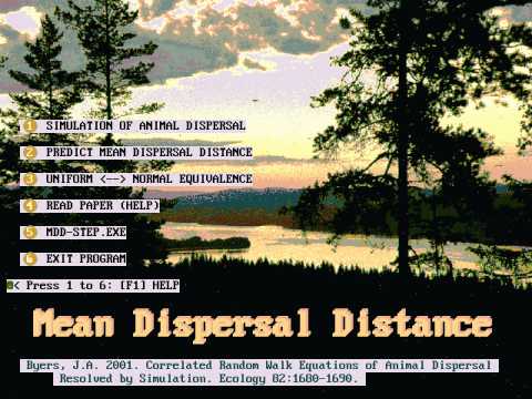
Opening screen of software for simulation and calculation of mean dispersal distance
Download MEAN-DD.ZIP Software?

---

Abstract Animal movement and dispersal can be described as a correlated random walk dependent on three parameters: number of steps, step size, and distribution of random turning angles. Equations of Kareiva and Shigesada use the parameters to predict the mean square displacement distance (MSDD), but this is less meaningful than the mean dispersal distance (MDD) about which the population would be distributed. I found that the MDD can be estimated by multiplying the square root of the MSDD by a three-dimensional surface correction factor obtained from simulations. The correction factors ranged from 0.89 to 1 depending on the number of steps and the variation in random turns, expressed as the standard deviation of the turning angles (SDA) about 0° (straight ahead). Corrected equations were used to predict MDDs for bark beetles, butterflies, ants, and beetles (based on parameters from the literature) and the nematode Steinernema carpocapsae (Weiser). Another equation from the literature finds the MDD directly, and this agreed with the MDD obtained by simulation at some combinations of SDA and numbers of steps. However, the equation has an error that increases as a power function when the standard deviation of turning angles becomes smaller (e.g., < 6° at 1000 steps or < 13° at 250 steps). Lower numbers of steps also increase the error. Equivalent values of AMT (angle of maximum turn) in uniform random models and of SDA in normal random models were found that allowed these two models to yield similar MDD values. The step size and turning angle variation of animal paths during dispersal and host and mate searching were investigated and found to be correlated; thus, use of different measured step sizes gives consistent estimates of the MDD.

---

Key words: bark beetle; Coleoptera; correlated random walk; dispersion; host searching; insect dispersal; mate searching; mean dispersal distance: Nematoda; Scolytidae; Steinernema carpocapsae; Steinernematidae.

---

INTRODUCTION

Prior to 1950, the dispersal of animals was attributed to a steady leakage of individuals out of an area, a forced exodus due to overcrowding, and accidental transport (Wellington 1979). The risks of dispersal were emphasized more often than the benefits, and population ecology usually ignored dispersal since it is difficult to observe. Insects and other animals often disperse from their brood habitat due to a lack of food resources, suitable mates, and te.rritories, or from the need to escape the local buildup of parasites and predators (Johnson 1969, Kennedy 1975, Southwood 1977, Wellington 1979, Root and Kareiva 1984, Ricklefs 1990). Evolution has favored life strategies that can take advantage of changing mosaics of suitable habitats (Cain 1985). Obligatory dispersal, an innate programmed dispersal regardless of current habitat conditions, also is adaptive if this prevents injury that otherwise would occur by staying in areas likely to rapidly deteriorate in resources and increase in competition.

The role of dispersal of animals in population ecology has been investigated from two directions: (1) theoretical analyses using diffusion models and (2) empirical studies that employ computer simulations (Turchin 1991). Increasingly, these two approaches have been compared or integrated (Kareiva and Shigesada 1983, Bovet and Benhamou 1988, Turchin 1991, Hill and Hader 1997, Byers i999, 2000). The advantage of equations as models is that they can be applied easily and provide nearly instantaneous answers. The disad- vantage is that equations are not often intuitive and usually difficult to verify. Simulations, on the other hand, always take much longer to produce results and require program software. However, the supposed va- lidity of equations may be corroborated or falsified by simulations that can be visualized on a computer screen. Often simulations are the only way to begin to understand natural processes that appear intractable to modeling by equations.

The well-known diffusion equation for two dimensions (Pielou 1977, Okubo 1980, Rudd and Gandour 1985) accurately predicts the density of organisms at any distance from the release point after a certain time or number of steps, but only for completely random walks. This type of random walk would have a uniform random distribution of turns with a maximum angle of turn (AMT) of 180° right or left. Insects and many other organisms do not exhibit truly random or Brownian movement but rather show correlated random walks in which the previous direction influences the direction of the next step (Fig. 1; Kitching 1971, Kareiva and Shigesada 1983, Bovet and Benhamou 1988, Byers 1991, 1996, 1999, 2000, Hill and Hader 1997). Here I want to consider whether it is possible to use a correlated random walk equation to accurately predict the mean distance of dispersal of a population of animals from a release point given any values for (1) the step size (or mean step size), (2) the number of steps, and (3) the distribution of possible random turning angles at each step. The mean distance of dispersal and variance can be found by simulation to check the validity of any such equation.

Patlak (1953) reports a modification of the Fokker-Planck equation that can predict densities of points at any distance and time for correlated random walks where the mean angle of turn is known. However, his Eq. 42 is extremely complex and thus has not been used in practice. Turchin (1991) took the Patlak equation for one dimension and "simplified" it in his work on patch density transitions. His equation is still complex and difficult to use, and it is not as yet applicable in two dimensions. The equation of Kareiva and Shigesada (1983) uses move lengths, turning angles, and total number of moves to calculate an expected mean square displacement distance (MSDD). However, the MSDD is not a meaningful distance since it is much larger than the mean dispersal distance (MDD), around which the population would be distributed (McCulloch and Cain 1989, Crist et al. 1992). Taking the square root of the MSDD only approximates the MDD, and, depending on the parameters used, can vary in its inaccuracy by up to 12%. The calculation of an MDD seems difficult as stated by McCulloch and Cain (1989) who derived an approximate formula which was again very complex to compute for a limited number of moves. However, a formula by Bovet and Benhamou (1988) claims to solve the MDD based on the mean vector length of turning angles, step size, and number of steps.

The first objective was to compare two models of simulated dispersal with regard to turning angles, (1) a uniform random distribution and (2) a normal random distribution, and see how the models affect the mean dispersal distance (MDD) and its variation. The second objective was to find correction factors that would correctly convert the mean square displacement distance of Kareiva and Shigesada (1983) to an MDD. Finally, the simulated results were used to test the formula of Bovet and Benhamou (1988) and show how it becomes increasingly inaccurate at low angular turning distributions and lower numbers of steps.

METHODS

Simulation of animal dispersal by correlated random walks
The algorithms for simulating animal movement in two dimensions follow the ideas of Skellam (1973) as described for computer (Kitching 1971, Kareiva and Shigesada 1983, Bovet and Benhamou 1988, Byers 1991, 1996, 1999, 2000). Modeled animals take steps with random angular deviations right or left from the former step's direction. The path of an animal is determined by first calculating the movement vector using polar coordinates from the former position based on the step size (or distance traveled in one second) and former direction plus the random angle of turn depending on the chosen angular distribution. Two types of turning angle models were employed (Fig. 1): (1) a uniform random distribution of angles within a left or right angle of maximum turn (AMT), or (2) a normal random distribution of angles with standard deviation (SDA). The random angles from a normal distribution are chosen proportional to their Gaussian probability (Walker 1985).

---

Fig. 1. Frequency distributions of turning angles for either a uniform random distribution (top) between -AMT and AMT (angle of maximum turn, ±60°) or a normal distribution (bottom) with 60° SDA (standard deviation of turning angles). An animal might take step 1 and then turn at random from the previous direction (dashed line), in this case a turn of 20° to the left.

---

A computer program was used for simulations with input parameters of (1) dispersal time (or number of steps in some cases), (2) mean speed and step size, (3) distribution range of turning angles (± AMT for uniform or SDA for normal distributions), (4) number of animals, and (5) the area length and width. All animals were released from the origin with initial directions chosen randomly (0° to 360°). All simulations and graphical analyses were done using QuickBASIC 4.5 (Microsoft 1988) and PostScript 2.0 (Adobe Systems 1990) programming languages unless otherwise noted.

Comparison of uniform and normal distributions of random turning angles
An equation of Kareiva and Shigesada (1983) calculates the expected mean square displacement, E(R²_n), when move lengths, turning angles, and total movies are known. The E(R²_n), here called the MSDD, can be calculated below assuming the random turning angles are about equally distributed right/left from the previous direction:



where L is the step size (since L is constant then E(L²) = E(L)² = L²), n is the number of steps, and c is the mean of the cosines of all possible turning angles (in radians) from a specified random distribution [g(theta)]:



Assuming a uniform distribution of random angles 6 between -AMT and AMT, the mean cosine value c can be found either by computer iteration or more accurately with the following integral (Mathcad 7, MathSoft [1997]):



where A = AMT. The value c for a normal distribution with a specified standard deviation (e.g., sigma = 10°) is found either by computer iteration or by integration (see Eq. 6 below):



Eqs. 3 and 4 were used to find equivalent values for AMT and SDA that should give similar MDDs in simulations.

Calculating mean dispersal disrtance (MDD)
The problem is now to use the mean square displacement distance (MSDD) of Kareiva and Shigesada (1983) from Eq. 1 using c from Eqs. 3 or 4 to find the MDD. A first approximation is to take the square root of the MSDD, but this may overestimate by up to 12.4% the actual MDD. In order to find correction factors that could by multiplied by the square root of the MSDD to obtain an MDD, simulations were performed where the number of steps and the AMT or SDA (0° to 60°) were varied. After each simulation run, an MDD was calculated from the mean of 1000 Euclidean distances from the start point to the final positions. These MDDs were divided by the square root of the MSDD calculated from the equations above with relevant parameters to yield correction factors. The correction factors depend on two variables, number of steps and distribution of turning angles, and thus are fit by surface equations in three dimensions (Mathcad 7, MathSoft [1997]).

An equation for the MDD was presented by Bovet and Benhamou (1988):



where



and SDA is as above but expressed in radians, with L and n as above. This equation was found to report values different from the corrected Kareiva and Shigesada equation or from simulation results. In order to describe which angular distributions and numbers of steps gave errors in excess of 1 % and 5%, stepwise calculations from 5 to 1000 steps at SDA in 0.06° increments from 0° to 30° at each step were done for the two equation types. Values were recorded when transitions in error limits occurred.

Using turning angles and steps of organisms to estimate MDD
The angular distributions of path segments and their lengths reported in the literature were used to estimate dispersal distances for various organisms. In addition, several hundretl insect-killing nematodes, Steinernema carpocapsae (Weiser) (Byers and Poinar 1982), were released from a central point on 1% ion agar covered with a film of carbon particles (india ink). After l8 h of dispersal at 20°C, the tracks were photographed, the slide scanned (Olympus ES-10; Olympus Optical, Tokyo, Japan), the image printed, and then coordinates along tracks recorded with a digitizing tablet (ACECAD D-9000; ACECAD, Taipei, Taiwan) connected to personal computer. A computer program in BASIC calculated the angles and distances between coordinates.

Effects of turning angles and step number on variation in dispersal distances
The mean dispersal distance from the origin is derived from the individual distances which have a variation that depends on both the turning angles and the total number of steps. The variation in distances can be expressed as the coefficient of variation (CV), which is the standard deviation (SD) as a percent of the mean. Simulations were used to find the relationship between the AMT or SDA and the cu of a population if the animals took either 180 or 3600 steps. Similarly, the relation between the number of steps and the CV was found for populations with AMT or SDA turning angles of 4° and 20° using logistic and Gompertz nonlinear regressions (STATISTICA, StatSoft [1997]; see formulas shown in Figs. 8 and 9).

Eftects of arbitrary path segmentation on calculating the MDD
In practice, a path of an organism is often segmented into steps based on constant distance or time and the turning angles measured between successive moves (as was done above for the nematode tracks). It might be that the choice of the step size or time unit would affect the estimated MDD. This was tested by generating the coordinates of a path of 2001 steps of 2 m each and random turning angles with an SDA of 30°. The path then was segmented into fewer steps by connecting every second, third, and so on, coordinates and measuring the resulting step sizes and angular turns (cosine of radian) by computer. These two values and the resulting number of steps were used to calculate the MDD using the equations derived in the results section.

RESULTS

Simulation of animal dispersal by correlated random walks
Simulations using different movement parameters were performed in order to test the equations for calculating mean dispersal distance (MDD) and mean square displacement distance (MSDD). The simulation models were validated in part by watching pixel movements on the computer screen that appeared to mimic natural dispersal of animals. Two models were used, with either a normal or uniform distribution of turning angles. These models when given equivalent parameters could produce similar density distributions of 1000 "bark beetles" released from a point source and "flying" for 1 h (Fig. 2). In these examples, beetles flew at 2 m/s (Byers 1996) and at each step of 2 m they could turn at random either left or right with an AMT (angle of maximum turn) of 10° (uniform) or with an SDA (standard deviation of turning angle) of 5.776° (normal). The SDA of the normal and the AMT of the uniform distributions were chosen appropriately to yield equivalent mean dispersal distances (MDD) as explained subsequently.

---

Fig. 2. Cell counts (nine-cell rolling mean) showing density distributions of 1000 simulated bark beetles after dispersal from a point source at the center of a 10 x 10 km grid for 1 h. Beetles flew at 2 m/s, and at each step of 2 m they could turn at random either left or right up to a maximum of 10° according to either a uniform random distribution (top), or according to a normal distribution of turning angles with a standard deviation of 5.776° (bottom). The MDD for the uniform (top) and normal (bottom) populations were similar, as expected, at 2054.4 ± 62.4 m (mean ± 95% CL) and 2137.0 ± 65.4 m, respectively.

---

The MDD for the uniform distribution was predicted at 2103.7 m (using the correction factor method, explained in Eqs. 8 and 9 below) while the simulated MDD was 2054.4 m (SD = 1008.4 m, CV = 49.08%). The MDD for the "equivalent" normal distribution was predicted to be 2130.8 m (correction factor method) or 2115.9 m (Bovet and Benhamou 1988) while the simulated value was 2137.9 m (SD = 1057.4 m, CV = 49.46%). The movement and distribution of "animals" in the two types of models appear nearly identical, although it is possible for a larger turn with the normal distribution.

Comparison of uniform arid normal distributions of random turning angles
The mean cosine of turning angles from a uniform distribution of angles decreases from 1 to 0 with an increase in AMT from 0° to 180° (Eq. 3, Fig. 3). In the case for a normal distribution, the mean cosine also decreases as the SDA is increased to 180°, but the curve is more sigmoid in shape (Eq. 4, Fig. 3).

---

Fig. 3. Mean cosine of turning angles possible at each step as a function of either a uniform or normal distribution of random turning angles. The uniform distribution had random angles between -AMT and AMT, while the normal distribution had a standard deviation (SDA) as indicated.

---

The question to solve is whether an organism that turns with a uniform random distribution of angles between left/right turns of, for example, an AMT of 10° might disperse to a mean distance identical to another type that has a normal random distribution of turns with perhaps an SDA of 5.8°. The value of SDA (a) that gives an equivalent c for a specified AMT is solved by combining Eqs. 3 and 4:



which is graphically represented by the curve shown in Fig. 4.

---

Fig. 4. Relation between standard deviation (SDA) of a normal distribution and AMT of uniform random distribution of turning angles yielding an equal mean cosine of turning angles (c of Kareiva and Shigesada 1983). The equation to calculate SDA (Y) from AMT (X) as shown (Eq. 5 in text) was found by equating the relations in Fig. 3 (Eqs. 3 and 4 in text).

---

However, an algebraic solution for AMT given SDA is not possible except by using iterative calculations such as with binary successive approximation. This method is employed in the computer program available in the Supplementary Materials. The relationship for SDA vs. AMT (Eq. 7, Fig. 4) was used to convert the AMT = 10° to an equivalent SDA = 5.776° to obtain the similar density distributions of simulated bark beetles after 1 h of flight (Fig. 2).

Calculating mean dispersal distance (MDD)
Simulations using various step sizes, and varying both the number of steps and the AMT or SDA (from 0° to 60°) stepwise, were used to calculate the MDD with the Pythagorean formula. The resulting MDD were compared to square roots of expected mean square distances based on Eqs. 1, 3, and 4. The comparisons showed that for a large number of steps and larger ttirning angles, the actual dispersal distance is ~89% of the square root of the expected MSDD. This proportion (MDD/SQRT(MSDD)) is called the correction factor (Fig. 5) since its multiplication by the square root of the expected MSDD gives the simulated MDD (equivalent to the natural MDD). The step size has no effect on the correction factor, but does scale the MDD.

---

Fig. 5. Correction factor as a three-dimensional surface function of the number of steps and either the ± AMT uniform random distribution or the normal random distribution (standard deviation, SDA) of possible turning angles taken at each step. The mean dispersal distance after some number of steps is obtained by multiplying the appropriate correction factor by the square root of the predicted mean square displacement distance (see Eqs. 8 and 9). Points represent means of four simulations of 1000 points each.

---

However, there is a complex interplay between the AMT or SDA (Y) and number of steps (X) on the correction factor which makes it necessary to describe it as a three-dimensional surface, especially at angles < 30° and steps < 5000 (Fig. 5).

The surface equation of the correction factor (Z) can be described reasonably well by a multivariate least squares cubic polynomial:

Z = aX3 + bX2 + cX + dX2Y + eXY + fXY2 + gY + hY2 + iY3 + j	(8)

where a = -2.191 X 10^-13, b = 4.472 X 10^-9, c = -3.31 X 10^-5, d = -1.803 X 10^-11, e = 4.611 X 10^-7, f = -2.095 x l0^-9, g = -0.01, h = 2.604 x 10^-4, i = -2.206 X 10^-6, and j = 1.043 for AMT and a uniform random distribution (Mathcad 7; MathSoft [1997]). However, the fit is best'over a limited range, therefore five constraints applied in order are needed:
(1) if AMT < 1° then interpolate Z between Y = 1° and 0° at X, i.e., Z_(x,y) = Z_(x,1) + (Z_(x,0) - Z_(x,1))(1 - Y), where Z_(x,0) is 1; (2) if AMT > 30° then Z = 0.89; (3) if AMT > 20 and steps > 2000, then Z = 0.89; (4) if Z > 1 then Z = 1; and (5) if Z < 0.89 then Z = 0.89. Eq. 8 and constraints also calculate correction factors for normal distributions of turning angles, where a = -1.772 X 10^-13, b = 3.823 X 10^-9, c = -2.786 X 10^-5, d = -2.657 X 10^-11, e = 5.515 X 10^-7, f = -3.253 X 10^-9, g = -0.012, h = 3.759 X 10^-4, i = -3.531 X 10^-6, and j = 1.028. Careful inspection of the correction factors from the two models, uniform and normal, does reveal small differences (Fig. 5).

In practice, if the mean step size is 2 m (L), 1000 steps are taken (n), and the AMT is 30° or 0.5236 radians, then c = 0.9549 from Eq. 3 and the expected MSDD is 169 752 m from Eq. 1 so the mean dispersal distance (MDD) is



where z = 0.89 from Eq. 8 and constraints. Five simulations with the same parameters and 1000 insects each gave a MDD of 364.0 ± 5.3 m (95% CL). This means that instead of using time-consuming and complex simulations to find the MDD, it can be calculated as accurately by the equations above with the mean step size, number of steps, and AMT or SDA.

Eqs. 5 and 6 (Bovet and Benhamou 1988) usually give nearly the same MDD as the application of the correction factor to the equations of Kareiva and Shigesada (I983). For example, using the parameters above and converting AMT = 30° to an equivalent SDA with Eq. 7 gives 17.40° or 0.304 radians, their equation predicts an MDD of 370.2 m (compared to 370.1 m for the correction factor method). Unfortunately, their equation becomes increasingly incorrect for turning angle distributions at smaller SDA, for example, at 1000 steps the error becomes apparent at an SDA < ~6° (Fig. 6).

---

Fig. 6. Comparison of MDD calculated from equation of Bovet and Benhamou (1988) with MDD calculated from corrected square root of MSDD (Kareiva and Shigesada 1983) and MDD from simulation as a function of SDA. The latter two MDD estimates are indistinguishable. Each point of the simulated data represents an MDD of 1000 organisms. All calculations are based on organisms taking 1000 steps of 2 m each.

---

A large range of SDA as well as lower numbers of steps give errors in excess of 1% and 5% (Fig. 7), indicating the Bovet and Benhamou equation should only be used for x, y values above the 1% shaded area (Fig. 7).

---

Fig. 7. Shaded areas represent x, y values that generate errors for the mean dispersal distance (MDD) using the Bovet and Benhamou (1988) equation that are in excess of 1% and 5%, as indicated, compared to simulated results or corrected square roots of MSDD (Kareiva and Shigesada 1983). Curves were generated by comparing differences in formulas by computer iteration of steps vs. SDA over the ranges as indicated.

---

Using turning angles and steps of organisms to estimate MDD
The twisting paths of organisms can be segmented into small steps of x, y coordinates and the angles between coordinates measured. The path is then described as segment lengths with a mean and variance as well as the distribution and mean of turning angles from the previous direction. In the simulations here, I have used the SDA or standard deviation in the expression of the turning angles from the previous direction. In addition to this way, other authors have used different values such as (1) the mean or variance of absolute angular deviation (AAD), (2) the mean vector length (r), and (3) the K value of turning angle concentration (Batschelet 1981, Cain 1985, Casas 1988, Wallin and Ekbom 1988, Turchin et al. 1991, Hill and Hader 1997, Kindvall et al. 2000). These different values can be converted to SDA. The relationship between SDA and an absolute angular deviation (AAD) was found by increasing the SDA in increments and taking some hundreds of random numbers from the appropriate distribution (Walker 1985) and determining the mean and SD of the AAD. This relationship is linear: mean of AAD = -0.31 + 0.8136(SDA) or SD of AAD = -0.2 + 0.611(SDA). However, this assumes that the data are normally distributed.

The mean vector length (r), a simple expression of path sinuosity, can be converted to SDA by solving Eq. 6:



with r not equal to 0.

The K value can be converted to SDA using table C in Batschelet (1981). SDA is expressed in degrees when using the correction factor method or in radians (e.g., SDA°/180*pi) for the exact method of Bovet and Benhamou (1988).

The MDDs of various populations of organisms after 1000 steps were calculated with Eqs. 5 and 6 using data from the literature, or from nematode tracks on agar, and converted or averaged when necessary to obtain a step size and SDA (Table 1). Both the equation of Bovet and Benhamou (1988) and the transformed MSDD equation (Eq. 9) gave essentially the same results (Table 1).

Table 1. Prediction of mean dispersal distance (MDD) after I000 steps for the nematode Steinernema carpocapsae and various insects (data from literature) based on mean step length and SDA.
Organism (study)	meam step length (N)	SDA (°)	MDD after 1000 steps (time)a
Nematode: Steinernema carpocapsae on 1% agar (original data)	0.3515 mm (1403)	19.66	5.76 cm (4.88 h)
Ant: Serrastruma lujae foraging (A. Dejean in Bovet and Benhamou 1988)	1.5 cm (664)	46.98	1.03 m (67.8 min)
Ant: Tapinoma nigerrimum foraging (Lopez et al. 1997)	2.68 cm (29)	33.7	2.56 m (33.3 min)
Darkling beetle: Eleodes extricata in grass (Crist et al. 1992)	4 cm	53.75b	2.42 m (83.3 min)
Ground beetle: Pterostichus melanarius (Wallin and Ekbom 1988)	1.28 m (86)	44.68c	92.62 m (10.42 d)
Butterfly: Pieris rapae ovipositing (Root and Kareiva 1984)	2.56 m (327)c	48.06c	172.44 m (5.56 h)
Butterfly: Euphydryas editha (Turchin et al. 1991)	7.16 m (140)	56.02b	415.5 m
Weevil: Hylobius abietis on sand (Kindvall et al. 2000)	8.72 cm (78)	23.99d	11.71 m (2.78 h)
Hymenopteran parasitoid: Pnigalio soemius (Casas 1988)	2 mm (55)	41.43d	15.59 cm
aBased on mean velocity bConverted from mean vector length (or mean cosine) with Eq. 11. cGenerated from histogram of turning angles or step sizes using random variates dConverted from absolute angular deviation (ADD), SDA = (ADD + 0.31)/0.8136.

However, as mentioned earlier, the equation of Bovet and Benhamou (1988) is incorrect at low turning angles. For example, if organisms take 1000 steps of 2 m each with a 2° SDA, then they predict an MDD of 3220 m (2000 m is the theoretical maximum). In Eq. 9, the corrected square root MSDD predicts an MDD of 1784 m while simulation gave 1796 m (N = 1000).

The expected number of steps (n) required to reach a certain MDD based on turning angles (r) and step sizes (L) is derived here from Eq. 5:



Also, the expected step size needed to reach a certain MDD based on the turning angle distribution and number of steps can be derived



The expected mean vector length of turning angles necessary to reach an MDD based on the step size and number of steps is determined by



and use Eq. 10 to convert r to SDA. Eqs. 11-13, derived from Bovet and Benhamou's equation, must be used with caution since they will be inaccurate at low numbers of steps or low angles of turn (as seen in Fig. 7). In this regard, the equation y = 2.29 + 5836.3/x, where y is the SDA and x is the number of steps, can be used to find SDA values below which an error > 1% will result (R² = 0.95).

Effects of turning angles and step number on variation in dispersal distances
The longer animals disperse away from a source and the larger their turning angles, the more variation is expected in their spatial distribution with time - but what are the precise relationships? The coefficient of variation (CV) of the population's spatial distribution is the standard deviation of dispersal distance as a percentage of the mean distance. After a certain number of steps the CV is near 0% if the animals proceed nearly straight ahead (low AMT or SDA) and increases as the variation in possible angular turns increases (Fig. 8).

---

Fig. 8. Coefficient of variation (SD x 100/mean) in the distances of dispersing individuals after taking either 180 or 3600 steps from the origin as a function of either a uniform or normal distribution of random turning angles taken at each step. The turns were either right or left from the former course using angles taken at random from a uniform distribution between -AMT and AMT (Fig. 1), or from a normal distribution with standard deviation (SDA) as indicated. Each point represents a mean of 1000 individuals. Logistic curves (equation in figure) fit the data well (R² > 0.99) in all cases.

---

In all cases, the relationships are logistic and increase toward the asymptote more rapidly at higher numbers of steps (Fig. 8). The maximum CV at the asymptote is probably the same for all combinations of steps and turning angles regardless of whether from a normal or uniform distribution, and is ~51% (Fig. 8).

If the number of steps is varied in increments instead, and turning angles are taken at random from normal and uniform distributions, then the cu begins near 0% and eventually reaches the same asymptote of 51 % regardless of the turning angles (Fig. 9).

---

Fig. 9. Coefficient of variation (SD X 100/mean) in the distances of dispersing individuals after taking various num- bers of steps from the origin as a function of either a uniform or normal distribution of random turning angles taken at each step. The turns were either right or left from the former course using angles taken at random from a uniform distribution between -AMT and AMT at either 4° or 20°, or from a normal distribution with standard deviation (SDA) as indicated. Each point represents a mean of 1000 individuals. Gompertz curves (equation in figure) fit the data well (R² > 0.99) in all cases.

---

The "slope" for smaller angle AMT and SDA turning distributions is less since the population, dispersing initially in an expanding ring, takes longer to become spatially randomized due to the relatively straight paths (Fig. 9). Surprisingly, the relationships are not sigmoid (or logistic) but can be fit well by nonlinear Gompertz regression (formula in Fig. 9).

Effects of arbitrary path segmentation on calculating the MDD
The segmentation of a 2001-step path into larger and larger segments consisting of multiples of the steps from 1 to 200 resulted in increasing mean step size and mean cosine of turning angles (Table 2). However, the increasing step size, decreasing numbers of steps, and decreasing mean cosine of angles covaried so that the MDD estimate was largely unaffected (Table 2). Further increases in the segmentation size finally did increase the variation in MDD estimates.

Table 2. Prediction of the mean dispersal distance (MDD) based on different segmentations of a 2001 step walk (2-m steps of 30° SDA) resulting in different numbers of steps, mean step sizes, and mean cosine of turning angles.
Steps (divisor)	Mean step size ± 1 SD	Mean cosine ± 1 SD	MDD
2000 (1)	2.000 ± 0	0.8710 ± 0.1737	303
1000 (2)	3.856 ± 0.203	0.8200 ± 0.2385	344
500 (4)	7.328 ± 0.654	0.6938 ± 0.3854	342
333 (6)	10.488 ± 1.278	0.5710 ± 0.4902	325
250 (8)	13.456 ± 2.165	0.4589 ± 0.5519	310
200 (10)	16.067 ± 3.061	0.3656 ± 0.5981	296
100 (20)	26.242 ± 8.159	0.1828 ± 0.7016	280
40 (50)	45.38 ± 20.17	0.1457 ± 0.6664	294
20 (100)	71.24 ± 32.20	0.0973 ± 0.6852	311
10 (200)	98.47 ± 63.15	0.0641 ± 0.7117	294
Note: The segmentations, after the first step, were done by connecting every coordinate, or every second or more as indicated (divisor) to obtain the number of steps.

DISCUSSION
Animal dispersal is often difficult to observe for any extended period of time. For example, flying bark beetles cannot be observed for more than a few meters, although marked beetles can be recaptured in pheromone-baited traps at various distances up to several kilometers from a release site (Byers 1999). For this reason, simulation is used to understand the effects of component processes and leads to hypotheses that can be tested both by simulation and in the field. Simulation of dispersal is considered here as virtual reality. This means that if organisms behave according to several assumptions, then the resulting simulated displacements are how real populations with the same movement parameters would perform. Thus, the model assumptions are crucial to the proper testing of hypotheses. In this regard, the graphical representation of organisms moving about on the computer screen is important to the intuitive analysis of the appropriateness of assumptions.

For simulation of animal dispersal and the correlated random walk equations, the assumptions are that the habitat must be rather homogeneous and that the organisms have similar and consistent behavior with time. This implies that the distributions of step lengths and turning angles do not change during the course of dispersal. Furthermore, consistent behavior means that the animals are not constrained by a home range or the need to return to a nest. Examples of homogeneous habitats would be sand (beaches, deserts), grass (prairies), or agricultural crops for walking animals. Habitats also might appear homogeneous to surface-swimming or flying organisms (many insects fly relatively unobstructed within a few meters of the ground). Even obstacles in a uniform to random pattern at a larger scale could be considered homogeneous. However, the obstacles would tend to reduce the mean dispersal distance (MDD) in proportion to their density and size. For example, simulated bark beetles flying under the forest canopy and avoiding tree trunks (at the size and density of 70-yr-old Norway spruce, Picea shies) flew 5% less far from the source over an hour than when unhindered (Byers 2000). This was because avoidance of tree trunks required an occasional increase in the beetle's turning angle about once every 67 m of flight (Byers 1996).

The angle of maximum turn (AMT) has been used in simulating animal movement because it is the most easy to implement (Byers 1991, 1993, 1996). Other models have used the variance or standard deviation of the normal distribution of turning angles (SDA) since these presumably better reflect movement of organisms (Cain 1985, Bovet and Benhamou 1988, Crist et al. 1992). However, the two models appear to give similar results when using equivalent values of AMT and SDA (Figs. 2 and 4). Byers (1991, 1993, 1996) found little difference between simulations using either a 5° or 30° AMT in causing similar proportions of a bark beetle population to find mates while walking, or susceptible host trees while flying, due to boundary effects. Nonetheless, increasing the AMT or SDA significantly reduces the search area of an individual. The relationship between the AMT and SDA was established (Fig. 4 and Eq. 7) to find values that produced dispersal patterns yielding equivalent MDDs in both models (Fig. 2). However, this does not mean the models are identical since the normal distribution allows turns of any angle, while the AMT limits the range.

This paper develops equations (Eqs. 8 and 9) that utilize the MSDD of Kareiva and Shigesada (1983) to find a mean dispersal distance (MDD) of a population moving outward from an origin for any set of movement parameters that include the turning angle distribution (SDA), mean step size, and number of steps. The MDD can also represent the mean displacement of organisms distributed at random or uniformly over an area. The MDDs from the equations are the same as those obtained by simulation but are more readily and rapidly calculated. The calculated MDD can serve as a comparison to field observations of MDD, or in prediction of expected population dispersal given knowledge of movement parameters.

Eqs. 1 and 2 (Kareiva and Shigesada 1983) which find the mean square displacement distance (MSDD) have the advantage that any distribution of turning angles, including Gaussian, can be used by finding the mean cosine of the turning angles. If the mean cosine from a chosen angular distribution can not be found by integration, then computer iteration methods are used. The angular distributions are assumed to be symmetrical about 0° or straight ahead. The MSDD is proportional to the number of steps or time (Kareiva and Shigesada 1983). However, the MSDD is not intuitively meaningful since it is considerably larger than the MDD; for example, an MSDD of 122500 m implies an MDD < 350 m. The MDD can be found approximately by taking the square root of MSDD, but the true value of MDD is up to 12.4% less, depending on the turning angles and number of steps. The MDD can be found precisely by multiplying correction factors (Fig. 5) from an appropriate three-dimensional surface equation by the square root of MSDD (Eqs. 1, 4, 8, and 9).

A formula that calculates the MDD directly was presented by Bovet and Benhamou (1988) as represented in Eqs. 5 and 6. These equations are less well known since their paper was about calculating the "sinuosity" of paths and they did not draw attention to the MDD prediction. Also, there appear to be some limitations for their equations, first the turning angle distribution, represented by r (the mean vector length) assumes a normal distribution. Even if another distribution could be used, r (equal to the mean cosine of turning angles) would have to be calculated. Second, the equations overestimate the MDD significantly at high r (or low turning angles). For example, a 2° SDA, 2-m mean step, and 1000 steps gives an MDD of 3220 m, which is much more than the maximum possible if animals go straight for 1000, 2 m-steps to disperse 2000 m out from the release point. The discrepancy between actual MDD (from simulation) and the MDD from Bovet and Benhamou (1988) is seen clearly in Fig. 6. Their MDD is related as a negative power of SDA (R² = 1) which becomes increasingly incorrect for decreasing turn angle variation. In fact, the error depends on both the SDA and the number of steps (Fig. 7). For example, at 100 steps a > 5% error begins for an SDA < 25°. This problem is avoided by the surface equation correction of the square root of MSDD.

The coefficient of variation (CV) in the distance of dispersing individuals after various numbers of steps from the origin was related logistically to increasing values of AMT or SDA distributions (Fig. 8) or as a Gompertz function to numbers of steps (Fig. 9). In both these figures, the CV appears asymptotic at ~51-52%. Bovet and Benhamou (1988) give the SD of the MDD as 0.52(MDD) which is the same as a CV of 52%. However, Figs. 8 and 9 show that the CV is not constant but ranges from 0 to 0.52 (or 52%), being lower at lower turning angles and lower numbers of steps, precisely when the Bovet and Benhamou equation is inaccurate.

In practice, a path of an organism is often segmented into steps based on constant distance or time, and the turning angles measured between successive moves. It would seem that the choice of the step size or time unit would affect the estimated MDD. In addition, a calculation of the MDD based on analysis of initial movement paths might be in error due to heterogenous environments or changes in behavior during dispersal (Crist et al. 1992, Johnson et al. 1992, Wiens et al. 1993). However, if there are no changes in the turning rate and step sizes, other than random variations as in the simulation models, then the value calculated for the MDD is surprisingly stable over a large range of segmentations of the path (Table 2). This implies that the precise segmentation of natural paths in homogeneous environments is not critical until very large steps are measured that obscure the path.

ACKNOWLEDGMENTS
The work was supported by a grant from the Swedish Agricultural and Forest Research Council (SJFR). Several reviewers, editors (F. Adler), and B. Holmqvist were helpful in revision of the manuscript. F. Adler provided the integrals used in Eqs. 3, 4, and 7 to replace iterative methods used in earlier drafts.

JOHN A. BYERS Department of Crop Science, Swedish University of Agricultural Sciences, Alnarp, Sweden. Present address: Chemical Ecology

---

LITERATURE CITED
Adobe Systems. 1990. PostScript 2.0. Adobe Systems, San Jose, California, USA.

Batschelet, E. 1981. Circular statistics in biology. Academic Press, London, UK.

Bovet, P, and S. Benhamou. 1988. Spatial analysis of animals' movements using a correlated random walk model. Journal of Theoretical Biology 131:419-433.

Byers, J. A. 1991. Simulation of mate-finding behaviour of pine shoot beetles, Tonucns pbtiperda. Animal Behaviour 41:649-660.

Byers, J. A. 1993. Simulation and equation models of insect population control by pheromone-baited traps. Journal of Chemical Ecology 19:1939-1956.

Byers, J. A. 1996. An encounter rate model for bark beetle populations searching at random for susceptible host trees. Ecological Modelling 91:57-66.

Byers, J. A. 1999. Effects of attraction radius and flight paths on catch of scolytid beetles dispersing outward through rings of pheromone traps. Journal of Chemical Ecology 25:985-1005.

Byers, J. A. 2000. Wind-aided dispersal of simulated bark beetles flying through forests. Ecological Modelling 125:231-243.

Byers, J. A., and G. O. Poinar, Jr. 1982. Location of insect hosts by the nematode, Neoaplectana carpocapsae, in response to temperature. Behaviour 79:1-l0.

Cain, M. L. 1985. Random search by herbivorous insects: a simulation model. Ecology 66:876-888.

Cases, J. 1988. Analysis of searching movements of a leafminer parasitoid in a structured environment. Physiological Entomology 13:373-380.

Crist, T. O., D. S. Guertin, J. A. Wiens, and B. T. Milne. 1992. Animal movement in heterogeneous landscapes: an experiment with Elodes beetles in shortgrass prairie. Functional Ecology 6:536-544.

Hill, N. A., and D. P Hader. 1997. A biased random walk model for the trajectories of swimming micro-organisms. Journal of Theoretical Biology 186:503-526.

Johnson, A. R., B. T. Milne, and J. A. Wiens. 1992. Diffusion in fractal landscapes: simulations and experimental studies of tenebrionid beetle movements. Ecology 73:1968-1983.

Johnson, C. G. 1969. Migration and dispersal of insects by flight. Methuen, London, UK.

Kareiva, P. M., and N. Shigesada. 1983. Analyzing insect movement as a correlated random walk. Oecologia 56:234-238.

Kennedy, J. S. 1975. Insect dispersal. Pages 103-119 in D. Pimental, editor. Insects, science and society. Academic Press, New York, New York, USA.

Kindvall, O., G. Nordlander, and H. Nordenhem. 2000. Movement behaviour of the pine weevil Hylobius abietis in relation to soil type: an arena experiment. Entomologia Experimentalis et Applicata 95:53-61.

Kitching, R. 1971. A simple simulation model of dispersal of anilnals among units of discrete habitats. Oecologia 7:95-116.

Lopez, R, S. G. Fungairino, J. M. Serrano, R J. Acosta, and P. Reunanen. 1997. Alloethic efficiency in the patrolling networks of a polytnorphic ant, Tapinoma nigerrimum (Hymenoptera: Formicidae). Journal of Insect Behavior 10:115-127.

MathSoft. 1997. Mathcad7. MathSoft, Cambridge, Massachusetts, USA.

McCulloch, C. E., and M. L. Cain. 1989. Analyzing discrete movement data as a correlated random walk. Ecology 70:383-388.

Microsoft. 1988. Microsoft QuickBASIC programming in BASIC. Microsoft, Redmond, Washington, USA.

Okubo, A. 1980. Diffusion and ecological problems: mathematical models. Springer-Verlag, Berlin, Germany.

Patlak, C. S. 1953. Random walk with persistence and external bias. Bulletin of Mathematical Biophysics 15:311-338.

Pielou, E. C. 1977. Mathematical ecology. John Wiley and Sons, New York, New York, USA.

Ricklefs, R. E. 1990. Ecology. W. H. Freeman and Company, New York, New York, USA.

Root, R. B., and P. M. Kareiva. 1984. The search forresources by cabbage butterflies (Pieris rapae): ecological consequences and adaptive significance of Markovian movements in a patchy environment. Ecology 65:147-165.

Rudd. W. G., and R. W. Gandour. 1985. Diffusion model for insect dispersal. Journal of Economic Entomology 78:295-301.

Skellam, J. G. 1973. The formulation and interpretation of mathematical models o.f diffusionary processes in population biology. Pages 63-85 in M. S. Bartlett and R. W. Hiorns, editors. The mathematical theory of the dynamics of biological populations. Academic Press, London, UK.

Southwood, T. R. E. 1977. Habitat, the templet for ecological strategies. Journal of Animal Ecology 46:337-365.

StatSoft. 1997. STATISTICA. Tulsa, Oklahoma, USA.

Turchin, P 1991. Translating foraging movements in heterogeneous environments into the spatial distribution of foragers. Ecology 72:1253-1266.

Turchin, P., E J. Odendaal, and M. D. Rausher. 1991. Quantifying insect movement in the field. Environmental Entomology 20:955-963.

Walker, R. S. 1985. Understanding computer science. Volume II. Texas Instruments Inc., Dallas, Texas, USA.

Wallin, H., and B. S. Ekbom. 1988. Movements of carabid beetles (Coleoptera: Carabidae) inhabiting cereal fields: a field tracing study. Oecologia 77:39-43.

Wellington, W. G. 1979. Dispersal and population change. Pages 11-24 in A. A. Berryman and L. Safranyik, editors. Dispersal of forest insects: evaluation, theory and management implications. Proceedings of the second International Union of Forestry Research Organizations conference, Washington State University, Pullman, Washington, USA.

Wiens, J. A., T O. Crist, and B. T. Milne. 1993. On quantifying insect movements. Environmental Entomology 22:709-715.

SUPPLEMENTAL MATERIAL
The software for simulation, MDD prediction, and analysis is available in ESA's Electronic Data Archive: Ecological Archives E082-019.